How to Add a Header Row in Excel: 5 Simplest Methods

Method 1: Insert a New Row and Create Column Labels (Simple and Universal)

Best for: when your data starts in Row 1 with no labelsor your spreadsheet has “mystery columns” that only one person understands.

How to do it (Windows / Excel for Microsoft 365)

1. Click the row number where you want the header to appear (usually Row 1).
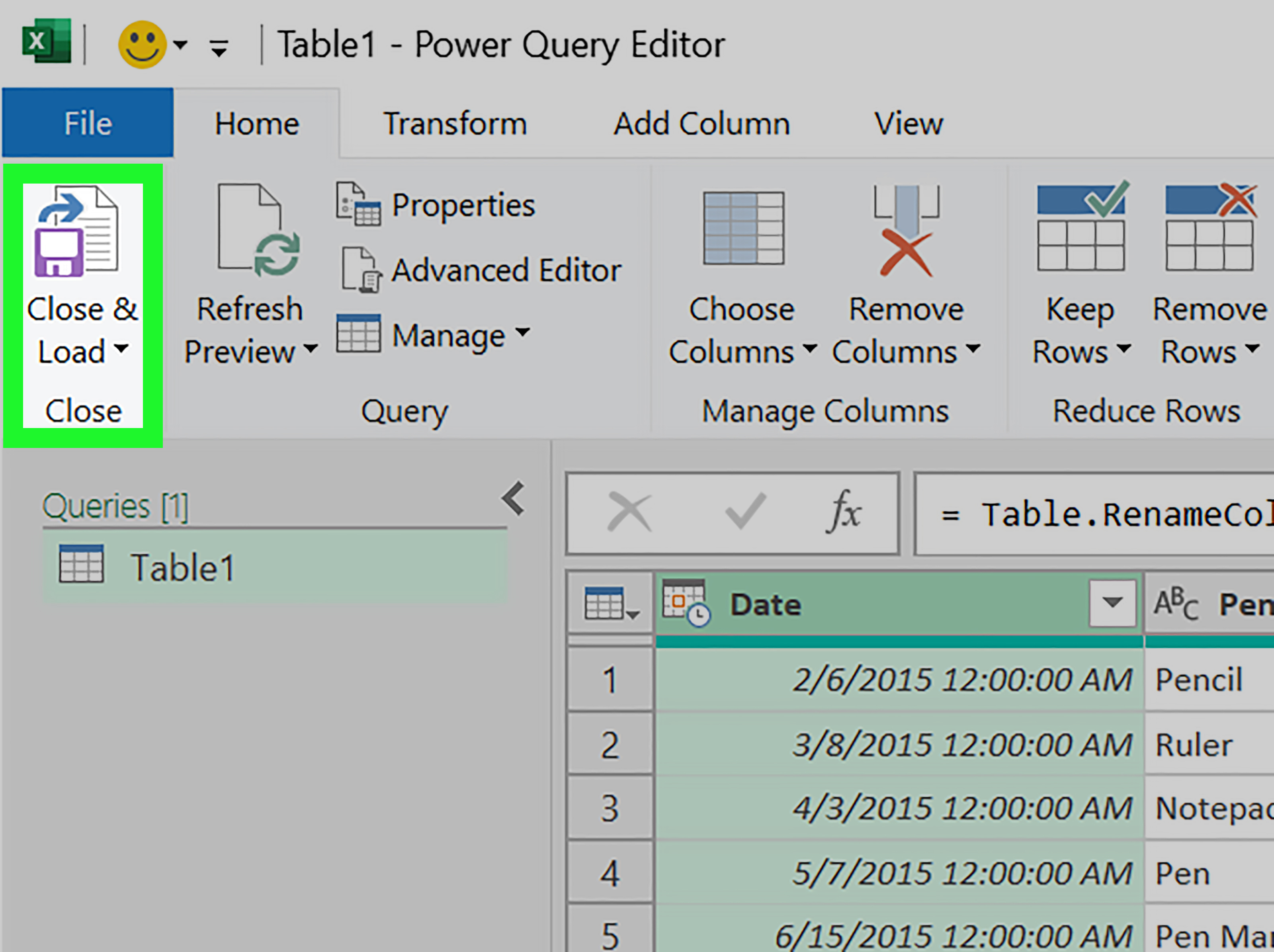
2. Go to Home > Insert > Insert Sheet Rows, or right-click the row number and choose Insert. ^[S2]
3. Type your column names into the new row (e.g., Date, Item, Quantity, Price, Total).

How to do it (Mac)

The idea is the same: select the row number, then use the Insert command (either from the Ribbon or a right-click menu). The labels you type become your header row.

A quick example

Let’s say you imported a CSV and it starts like this:

Insert a new Row 1 and label it:

Now your sheet is readable, sortable, and less likely to cause workplace dramatic readings.

Pro tips for Method 1

• Make headers obvious: bold text, a subtle fill color, and Wrap Text for long labels.
• Avoid merged cells in headers if you plan to sort/filter. Merged cells are the glitter of spreadsheets: they spread and never fully leave.
• Keep header names short but specific: “Total” is good; “Thing” is… a cry for help.

Method 2: Convert Your Data to an Excel Table (Ctrl+T = Instant Upgrade)

Best for: datasets you’ll sort, filter, expand, summarize, or generally treat like something important.

Turning a range into an Excel Table is one of the fastest ways to make a header row “official.” Tables come with built-in header formatting, filter drop-downs, structured references, and auto-expanding ranges. Plus, the Table feature lets you toggle the header row on/off if needed. ^[S3][S4]

Steps (Windows / Mac)

1. Click any cell in your dataset (or select the full range).
2. Press Ctrl+T (Windows) or Command+T (Mac), or use Insert > Table.
3. In the dialog box, confirm the range is correct.
4. If your first row already contains labels, check My table has headers. If it doesn’t, leave it unchecked and Excel will create generic headers you can rename. (Then rename them immediately. “Column1” is not a lifestyle.)

Turn the Table header row on/off

1. Click anywhere inside the table.
2. Open the Table Design tab.
3. Check or uncheck Header Row in Table Style Options. ^[S3][S4]

Why Tables are a big deal (quick analysis)

• Cleaner sorting/filtering: Excel recognizes the header row and uses it for menus and criteria.
• Auto-expanding: Add a new row under the table and formulas/formatting often carry down.
• Readable formulas: Instead of =SUM(D2:D200), you might see structured references that clearly tie to column names.

When not to use a Table: If your sheet is a highly customized layout (dashboards, forms, or “this looks like a poster” spreadsheets), a Table can feel restrictive. In that case, Method 1 + Method 3 is usually enough.

Method 3: Freeze the Header Row (So It Stays Visible While You Scroll)

Best for: long spreadsheets where you keep forgetting what Column H represents (and you don’t want to scroll back up like it’s a fitness routine).

Freezing panes locks rows/columns in place while the rest of the sheet scrolls. Excel freezes the rows above and columns to the left of the selected cell. ^[S1]

Freeze just the top row

1. Go to View.
2. Select Freeze Panes.
3. Choose Freeze Top Row. ^{[S9][S10][S11]}

Freeze multiple header rows (great for multi-line labels)

1. Click the first cell below the header area you want to keep visible.
2. Go to View > Freeze Panes > Freeze Panes. ^[S1]

Example: If your headers span Rows 1–2, click a cell in Row 3 (like A3), then Freeze Panes.

Unfreeze (if you froze the wrong thing)

Go to View > Freeze Panes > Unfreeze Panes. ^[S1]

Practical note: Freeze Top Row is fast, but if your header is not in Row 1 (for example, you have a title area above), use Freeze Panes from a selected cell to define exactly what stays visible.

Method 4: Repeat the Header Row on Every Printed Page (Print Titles)

Best for: reports that will be printed or saved as PDFs where every page should show the column labels.

Freezing helps on screen. Printing is different: you want the header row to repeat at the top of each printed page. That’s what Print Titles is for. ^[S5][S6]

Steps

1. Go to Page Layout.
2. Click Print Titles (in the Page Setup group). ^[S5]
3. On the Sheet tab, find Rows to repeat at top.
4. Enter the row reference, like $1:$1 to repeat Row 1. For two header rows, use $1:$2. ^[S6]
5. Click OK, then preview before printing.

If “Print Titles” is grayed out

• You might be actively editing a cell (press Enter/Esc to exit edit mode). ^[S6]
• Some setups require at least one printer configured for certain print settings to become available. ^[S6]

Why this matters: Without repeating headers, Page 2 becomes a guessing game. And in the Excel Olympics, guessing games are how spreadsheets win gold in confusion.

Method 5: Add Filter Drop-Downs to Your Header Row (Data > Filter)

Best for: quickly making your header row interactivesort and filter without building anything fancy.

Filtering works best when your data has a clear header row. When you turn on filters, Excel adds drop-down arrows to the header cells so you can filter by values, text rules, number rules, and more. ^[S7][S8]

Turn filters on

1. Click any cell inside your data range.
2. Go to Data > Filter. ^[S7]
3. Use the header arrows to sort or filter the column. ^[S7][S8]

Keyboard shortcut (because your mouse deserves fewer miles)

Toggle filters on/off with Ctrl+Shift+L (Windows). ^[S12]

Mini example: filter a sales sheet

If your header row has Region, click the filter arrow in that column and select only “West.” Now Excel shows just the matching rowsno copying, no deleting, no “temporary” edits that become permanent because you forgot.

Bonus tip: If you convert your range to a Table (Method 2), filter arrows usually come along for the ride automaticallyTables and Filters are basically best friends.

Header-Row Best Practices (Small Choices, Big Sanity)

1) Use clear, consistent names

Pick a naming style and stick to it: “Order Date” vs “Date Ordered” vs “When It Happened” is how a spreadsheet becomes a choose-your-own-adventure novel.

2) Keep headers to one row when possible

Multi-row headers can look nice, but they can complicate sorting/filtering unless you’re careful. If you truly need multiple rows (e.g., grouped categories), consider freezing multiple rows (Method 3) and using a Table only for the main data grid below.

3) Avoid blank rows/columns inside the dataset

Excel treats blank rows as natural “stopping points” for many features. If you want clean filtering and pivoting later, keep the data range continuous.

4) Format for readability, not decoration

• Bold headers and use a subtle background fill.
• Turn on Wrap Text if labels are long.
• Consider Center alignment for short headersbut don’t force it if it hurts scanning.

5) Make it “sticky” in the right way

If your biggest pain is scrolling, freeze the header (Method 3). If your biggest pain is printing/PDFs, repeat it with Print Titles (Method 4). If your biggest pain is finding anything, turn on Filters (Method 5). Different problems, different capes.

Troubleshooting: Common Header Row Problems (and Fixes)

Problem: Sorting includes my header row

Fix: Make sure Excel recognizes your headers. Converting to a Table (Method 2) is the most reliable. If you’re using Sort on a range, check the sort dialog for an option like “My data has headers” (wording varies by version), then retry.

Problem: Filters don’t show up or the arrows are weird

Fix: Click inside the range and re-apply Data > Filter. Filters attach to a range, so blank rows/columns or scattered data can confuse what Excel thinks the list is. ^[S7][S8]

Problem: I froze the wrong row (oops)

Fix: Unfreeze panes, then freeze again correctly. Freezing is based on the selected cell: rows above and columns left get locked. ^[S1]

Problem: “Print Titles” is grayed out

Fix: Exit cell edit mode and verify you can access printing features (some environments need a printer configured). ^[S6]

Problem: My header row wraps into a tall monster row

Fix: Shorten labels, widen columns, or use concise naming (“Unit Price” instead of “Price Per Individual Item In USD”). Wrap Text is greatuntil it becomes a novel.

Real-World Experiences & Lessons (Extra )

Header rows feel “basic” until you live through a spreadsheet horror storythen suddenly they’re your favorite safety feature. In real-world workbooks (the ones that have been emailed around for years and carry a faint aura of panic), header rows tend to fail in the same predictable ways. Here are the most common situations people run into, plus what actually helps.

1) The “I’ll remember what Column G is” phase

It starts with confidence. Column G is obvious. Everyone knows Column G is “Status,” right? Two weeks later, Column G is either Status, Stage, State, or “Something we stopped using but forgot to remove.” The fix is boring but powerful: name the column clearly, keep it consistent, and don’t be afraid to add a short note in a nearby cell if a label needs extra context. If it’s a Table (Method 2), the header becomes even more important because it shows up in filter menus and structured references. ^[S3]

2) The “pretty header” trap

Many spreadsheets try to look like a report: merged title cells, multi-row labels, decorative spacing, maybe a little clipartbecause why not. The problem is that sorting and filtering want a clean grid. If you need the report look, consider keeping a neat data table (with a normal header row) on one sheet and building your pretty summary on another sheet. Freeze your header (Method 3) so the data stays readable, and use Print Titles (Method 4) for any printed output. ^[S1][S6]

3) The “filter broke my brain” moment

Filtering is amazinguntil someone filters a column, forgets it’s filtered, and then announces, “We only have 12 orders this month.” (Cue dramatic music.) A reliable header row makes filter state easier to spot because the header arrows change appearance when filtered. Turning on filters intentionally (Method 5) is better than accidentally filtering random ranges. If the dataset matters, making it a Table helps even more because the filter controls live with the table and expand with it. ^[S7][S8][S3]

4) Printing: where spreadsheets go to become confusing

On screen, you can scroll back to Row 1 to remember what a column means. On paper or PDF, Page 2 is where meaning goes to disappear. The simplest printing upgrade is setting Print Titles so the header row repeats on every page (Method 4). It takes about 20 seconds and saves you from the “Page 3 Mystery Columns” detective arc. ^[S5][S6]

5) The “hand-off spreadsheet” reality

Most spreadsheets eventually get shared. Once that happens, your header row becomes a user interface. Great headers are like good road signs: clear, predictable, and not trying to be funny at the wrong time. (You can save humor for the sheet name. “Final_Final_RealFinal.xlsx” is comedy gold.) The best hand-off setup is usually: insert/clean headers (Method 1), convert to Table (Method 2) for structure, freeze top row (Method 3) for navigation, and use filters (Method 5) for quick searching. It’s not flashybut it’s the Excel equivalent of wearing a seatbelt and keeping snacks in the car. Sensible. Life-saving.

Wrap-Up

If you want the simplest path, here’s the no-drama combo:

• Add or fix the header row (Method 1).
• Convert to a Table if the data will grow or be analyzed (Method 2).
• Freeze the header so it stays visible while you scroll (Method 3).
• Repeat headers when printing for clean PDFs and reports (Method 4).
• Turn on filters to find things fast (Method 5).

Do that, and your spreadsheet becomes less of a “where am I?” experience and more of a “wow, I can actually work with this” moment.